Linear Regression

How Does Linear Regression Work?

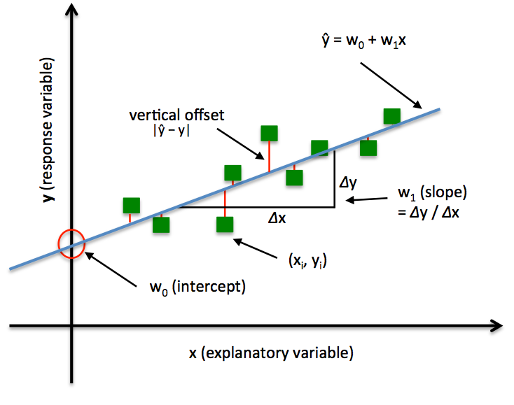
Linear regression is a statistical technique used to establish a relationship between a dependent variable and one or more independent variables. The goal of linear regression is to find the best-fit line that describes the linear relationship between the variables.
In simple linear regression, there is only one independent variable, and the goal is to predict the value of the dependent variable based on that variable. The equation for a simple linear regression is y = mx + b, where y is the dependent variable, x is the independent variable, m is the slope of the line, and b is the y-intercept.

In multiple linear regression, there are multiple independent variables, and the goal is to predict the value of the dependent variable based on those variables. The equation for multiple linear regression is y = b0 + b1x1 + b2x2 + ... + bnxn, where y is the dependent variable, x1, x2, ..., xn are the independent variables, b0 is the y-intercept, and b1, b2, ..., bn are the slopes of the line for each independent variable.

The process of linear regression involves fitting the data to the line of best fit using a method called the least-squares method. This involves minimizing the sum of the squared differences between the predicted values and the actual values.

Linear regression is commonly used in various fields, such as economics, finance, social sciences, and engineering, to analyze and predict the relationship between variables.
Linear regression simply means fitting a straight line in the given data set.

There are certain types involved in developing a linear regression model.

1. Data Gathering and Preprocessing
2. Fitting Data to the Model
3. Determining Cost Function
4. Minimize the error using Gradient Descent

Hypothesis function for Simple Linear Regression :

                                     y = mx + b

 Here we know that,

• m = Slope

• X = Independent Variable

• b = x-intercept

How to Fit a Straight Line to the Data?

Let us consider a random value for m (slope) and b (x-intercept) and predict y values by plugging all the values of x into the equation. After this, find errors for all the predicted y values.

Now, we use something called the Cost function which is also known as Mean Squared Error to find the average error. Now again we randomly choose another value for m and b
again repeat the steps mentioned above. We do this until we have the best-fitted straight line
(i.e) MSE or error should be minimum.
Doing this manually is very hard, So, we use gradient descent to minimize the error obtained in the cost function. This algorithm can be used to minimize any function.

Steps for Fitting a Straight Line:

1. choose random values for m and b
2. Predict y outputs
3. Find cost Function
4. Use gradient descent to minimize cost Function

Cost Function:

                                A cost function is a mathematical function used to quantify the error or loss between the predicted values and the actual values in a machine learning model. The goal of a machine learning model is to minimize the cost function, which means reducing the error between the predicted and actual values.

                        MSE = 1/n * sum((y - y_pred)^2)

where y is the actual value, y_pred is the predicted value, and n is the number of data points.

Gradient Descent:

Gradient descent is a popular optimization algorithm used in machine learning to find the optimal values of the parameters that minimize a cost function. The algorithm works by iteratively adjusting the parameters of the model in the direction of the negative gradient of the cost function until the optimal values are reached.

The gradient descent algorithm starts with an initial guess for the parameters of the model. The cost function is then evaluated for the current values of the parameters, and the gradient of the cost function is computed. The parameters are then updated by subtracting the product of the gradient and a learning rate from the current values of the parameters. The learning rate is a hyperparameter that determines the size of the step taken in each iteration.

The algorithm continues to iterate until the cost function converges to a minimum. There are two types of gradient descent: batch gradient descent and stochastic gradient descent.

The equation for the gradient descent algorithm is as follows:

θj = θj - α * ∂J/∂θj

where:

• θj is the jth parameter of the model that we want to optimize
• J(θ) is the cost function that we want to minimize
• α is the learning rate, which determines the step size in each iteration
• ∂J/∂θj is the partial derivative of the cost function with respect to the jth parameter.

The algorithm starts with an initial guess for the parameters θ, and then iteratively updates the parameters by subtracting the product of the learning rate α and the partial derivative of the cost function with respect to the parameters ∂J/∂θj from the current values of the parameters θ.

The partial derivative ∂J/∂θj measures the rate of change of the cost function with respect to the jth parameter. It tells us how much the cost function will change if we change the value of the jth parameter.

The goal of the gradient descent algorithm is to find the values of the parameters that minimize the cost function J. By iteratively adjusting the parameters in the direction of the negative gradient of the cost function, the algorithm moves towards the minimum of the cost function, where the gradient is zero.

The choice of learning rate α is important in the gradient descent algorithm, as it determines the step size in each iteration. If the learning rate is too large, the algorithm may overshoot the minimum and fail to converge. If the learning rate is too small, the algorithm may take too many iterations to converge. The learning rate is usually set through trial and error or by using a validation set to tune the hyperparameters.